How an LLM works, read straight from the file. A slide course through Qwen3-Coder in Netron.

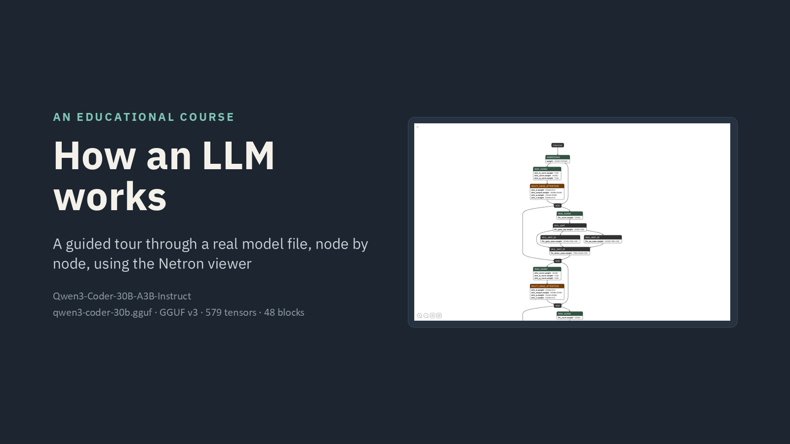
Most explanations of how a language model works start with the maths and stop before the file. This one goes the other way. The slides above open a real model, the 18 GB Qwen3-Coder-30B-A3B build that runs locally through Ollama, in Netron, a free offline viewer that draws any model file as a graph. Everything on every slide is a screenshot of that file. The head counts, the expert counts, the tensor shapes: none of it is a diagram somebody drew, it is the design, read off the artefact.

Click the deck to turn the pages, or use the arrow keys. The original PowerPoint is linked under it if you want to teach from it.

This article walks the same route as the slides, so you can read it alongside them or instead of them.

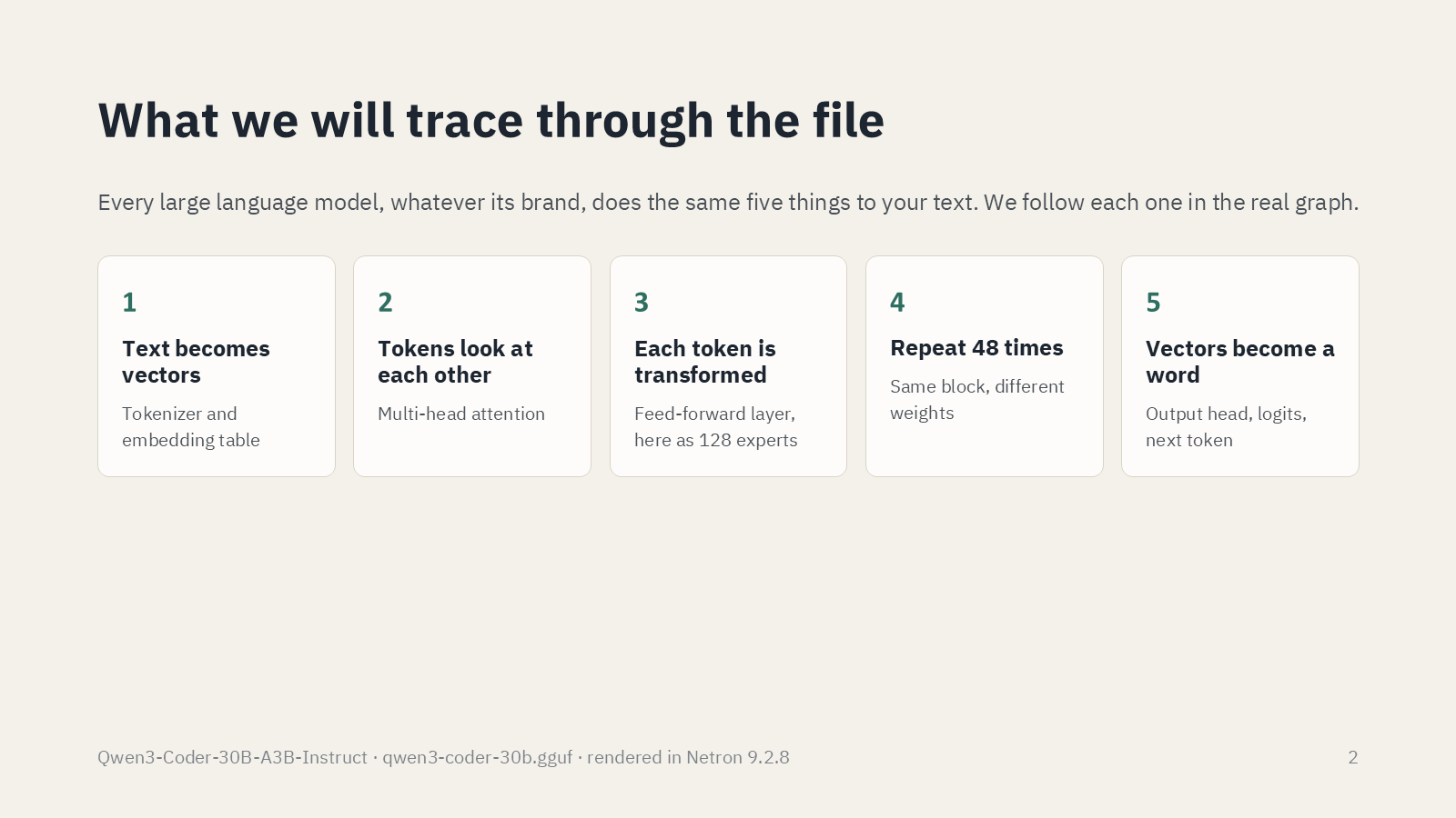
The five things every model does

Whatever the brand, a large language model does five things to your text. GPT, Llama, Claude and Qwen all follow the same shape. What differs is the size of each stage and a handful of design choices, two of which this particular file makes visible.

• Text becomes vectors. A tokenizer and an embedding table.
• Tokens look at each other. Multi-head attention.
• Each token is transformed. A feed-forward layer, which in this model is split into 128 experts.
• Repeat 48 times. The same block, with different weights each time.
• Vectors become a word. An output head, a score for every token in the vocabulary, one pick.

The rest of this piece takes them in order.

The file describes itself

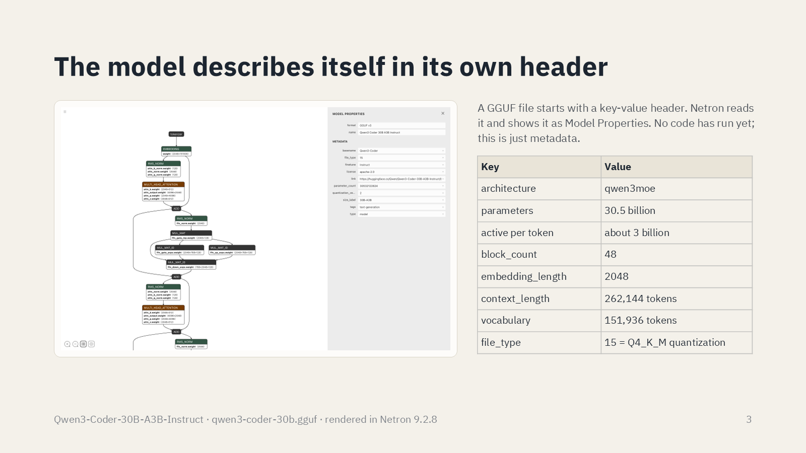
A GGUF file begins with a key-value header, and Netron shows it as the model's properties before a single calculation has run. Two numbers from that header matter for everything that follows. The embedding length is 2048, which is the width of every vector that flows through the network. The block count is 48, which is how many times the transformer block repeats.

The name is a third clue. 30B-A3B means 30 billion parameters stored and about 3 billion used for any single token. Slide 9 explains how that is possible.

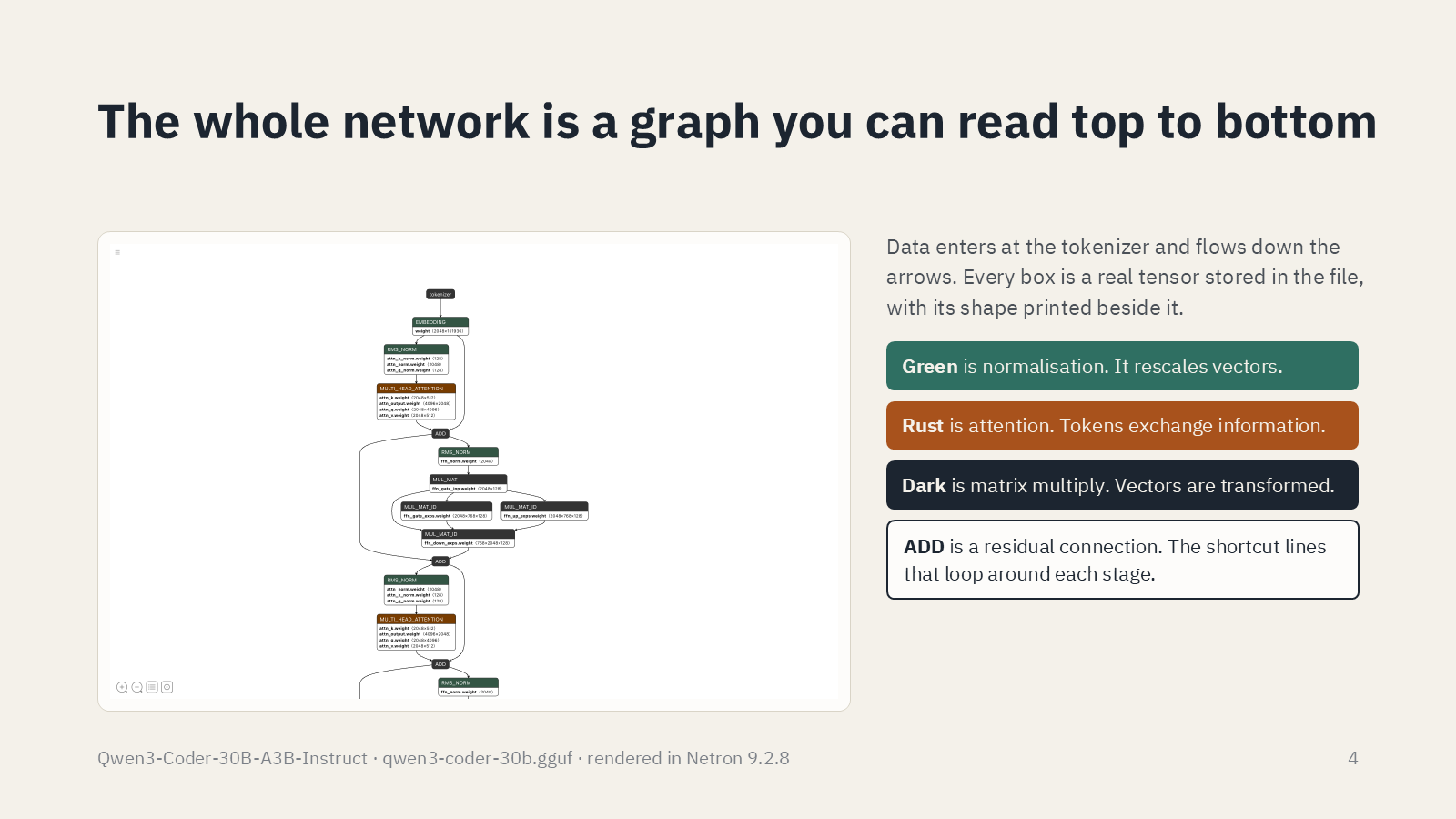
Zoomed out, the whole network is a graph you can read from top to bottom. Data enters at the tokenizer and flows down the arrows. Every box is a real tensor in the file with its shape printed beside it. Netron's colours are its own convention: green is normalisation, rust is attention, dark boxes are matrix multiplies, and the small ADD nodes are residual connections, the shortcut lines that loop around each stage. Give it a minute before reading on. The repeating pattern is visible before anyone names it.

Step 1: text becomes numbers

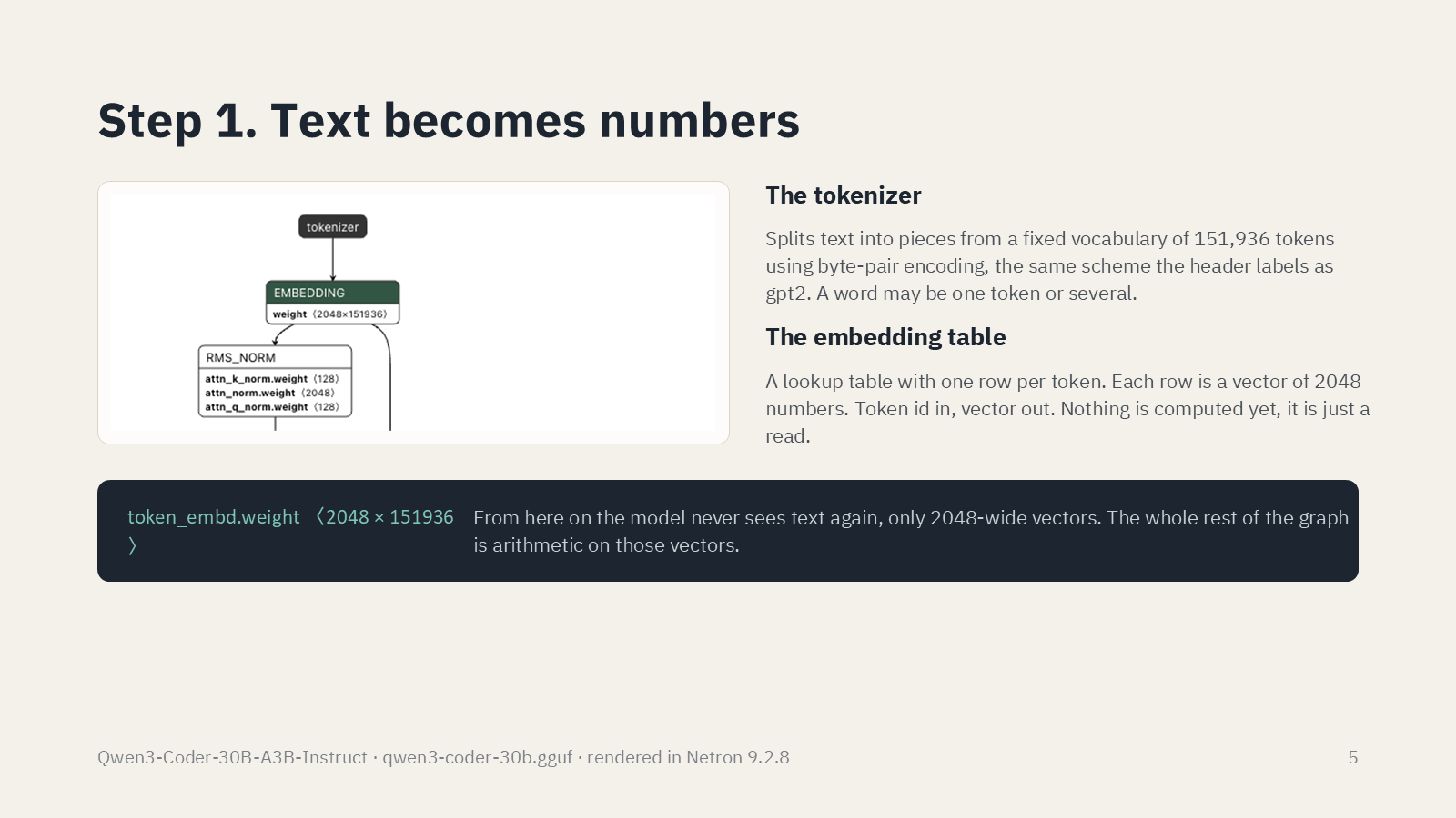
The tokenizer splits text into pieces from a fixed vocabulary of 151,936 tokens, using byte-pair encoding, the scheme the header labels as gpt2. A word may be one token or several.

The embedding table is a lookup: one row per token, each row a vector of 2048 numbers. Token id in, vector out. Nothing is computed here, it is a read. The tensor is called token_embd.weight and its shape, 2048 by 151,936, is about 311 million numbers on its own. It appears at both ends of the graph, because the same table that looks a word up at the start is used to score every word at the end.

From this point the model never sees text again. Everything downstream is arithmetic on 2048-wide vectors.

One block: two stages, each wrapped in a shortcut

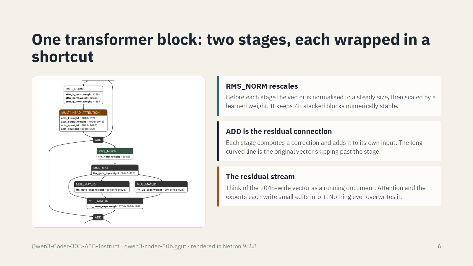
Before each stage an RMS_NORM node rescales the vector to a steady size and multiplies it by a learned weight. That is what keeps 48 stacked blocks numerically stable.

Each stage then computes a correction and adds it to its own input. The ADD node is the residual connection, and the long curved line on the graph is the original vector skipping past the stage. Trace the two shortcuts on slide 6: the first leaves just after the embedding and re-enters at the first ADD, skipping attention; the second leaves after that ADD and re-enters at the second, skipping the experts.

A useful way to hold this: the 2048-wide vector is a running document. Attention and the experts each write small edits into it. Nothing ever overwrites it. The idea came from image models in 2015, and it is the reason very deep networks can be trained at all.

Step 2: attention

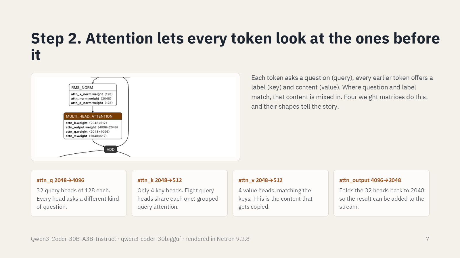
Each token asks a question, called a query. Every earlier token offers a label, the key, and some content, the value. Where a question and a label match, that content is mixed in. Four weight matrices do this, and their shapes tell the story of a design decision.

• attn_q takes 2048 to 4096: 32 query heads of 128 each. Every head asks a different kind of question.
• attn_k takes 2048 to 512: only 4 key heads. Eight query heads share each one.
• attn_v takes 2048 to 512: 4 value heads, matching the keys. This is the content that gets copied.
• attn_output takes 4096 back to 2048, so the result can be added to the stream.

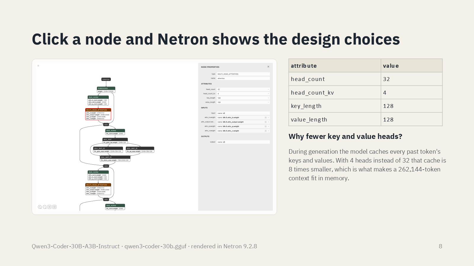
The arithmetic is checkable by anyone: 4096 divided by 128 is 32, and 512 divided by 128 is 4. Click the attention node and Netron prints the same figures as attributes, head_count 32 and head_count_kv 4, along with the exact tensor names, blk.0.attn_q.weight and so on. The blk.0 prefix means block zero, and every one of the 48 blocks carries its own copy of these four matrices.

Why fewer key and value heads? During generation the model caches every past token's keys and values. With 4 heads instead of 32 that cache is eight times smaller, and that is what lets a 262,144-token context fit in memory. This is grouped-query attention, and it is why the model's headline context length is a claim you can verify from the file rather than take on trust.

Attention in a language model is causal: a token can only look backwards. That constraint is what makes generating one token at a time possible.

Step 3: the feed-forward layer, as 128 experts

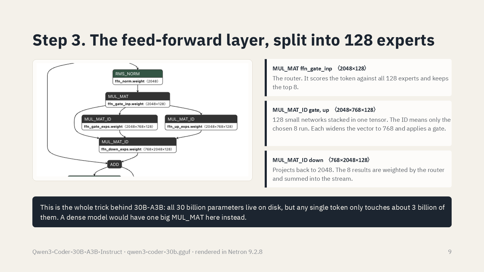
In a dense model the second stage of each block is one large matrix multiply. Here it is three nodes and a trick.

• ffn_gate_inp, a 2048 by 128 matrix, is the router. It scores the token against all 128 experts and keeps the top 8.
• ffn_gate_exps and ffn_up_exps, each 2048 by 768 by 128, are 128 small networks stacked in one tensor. The node type is MUL_MAT_ID, and the ID is the point: only the chosen 8 run. Each widens the vector to 768 and applies a gate.
• ffn_down_exps, 768 by 2048 by 128, projects back to 2048. The 8 results are weighted by the router and summed into the stream.

That is the whole of 30B-A3B. All 30 billion parameters live on disk, and every one of them has to be in memory, but any single token touches about 3 billion. The header keys are expert_count 128 and expert_used_count 8. The feed-forward stage is where most of a model's factual knowledge is thought to live, so splitting it into experts is a way of holding more knowledge without paying for all of it on every token. The trade-off is memory, not compute: the full 18 GB is resident either way.

Step 4: the same block, 48 times

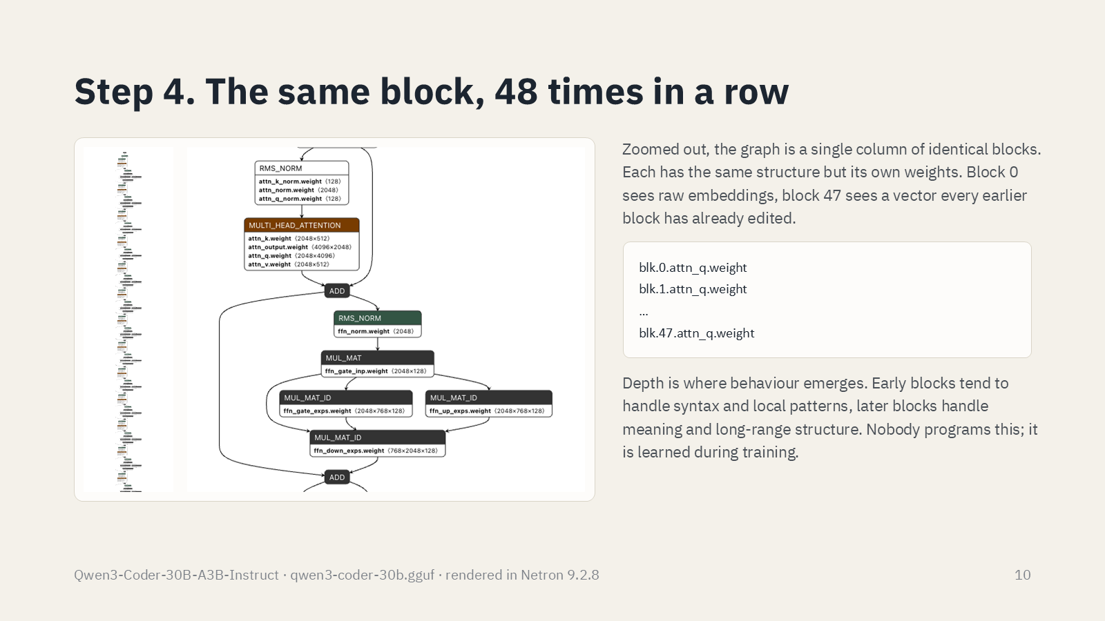
Zoomed all the way out, the graph is a single column of identical blocks. Each has the same structure and its own weights. Block 0 sees raw embeddings. Block 47 sees a vector that every earlier block has already edited.

Depth is where behaviour emerges. Early blocks tend to handle syntax and local patterns, later blocks meaning and long-range structure. Nobody programs that division; it is learned.

An exercise the deck sets, and one worth doing: count the tensors in one block in Netron. There are 12. Forty-eight blocks of 12 plus the 3 shared tensors is 579, which is the number the header reports.

Step 5: vectors become a word

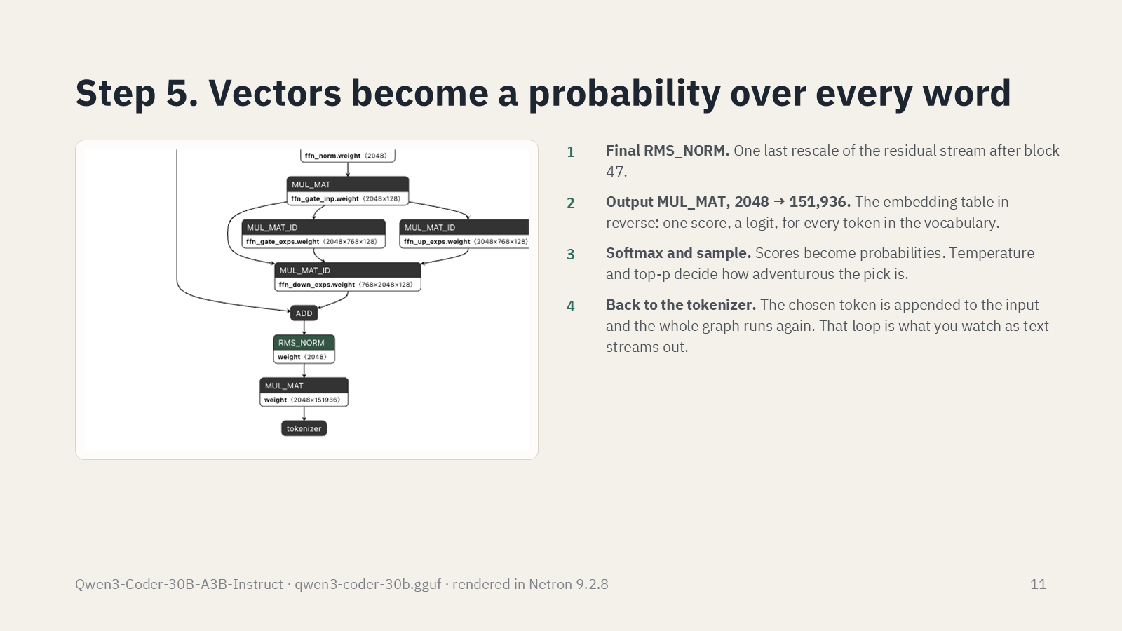
After block 47 there is one last RMS_NORM, then an output matrix multiply from 2048 to 151,936: the embedding table in reverse, producing one score, a logit, for every token in the vocabulary. Softmax turns the scores into probabilities. Temperature and top-p, the two settings every chat app exposes, decide how adventurous the pick is, and this is the exact place in the pipeline where they act.

Then the chosen token is appended to the input and the whole graph runs again. The arrow at the very bottom of Netron's graph, back up to the tokenizer, is the generation loop, and it is what you watch as text streams out. The model produces exactly one token per full pass and knows nothing about the sentence it is about to write.

Why 30 billion parameters fit in 18 gigabytes

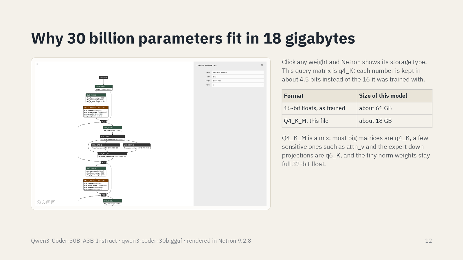
Click any weight and Netron shows its storage type. The query matrix on slide 12 is q4_K: each number is kept in about 4.5 bits instead of the 16 it was trained with. The Q4_K_M build is a mix. Most large matrices are q4_K, a few sensitive ones such as attn_v and the expert down projections are q6_K, and the tiny norm weights stay as full 32-bit floats.

Thirty and a half billion parameters at two bytes each is 61 GB. Quantised, the file is 18 GB, and that arithmetic is the whole reason a model of this class runs on a laptop. The quality loss at 4 bits is small but not zero; heavier quantisation such as Q2 degrades noticeably.

The whole forward pass

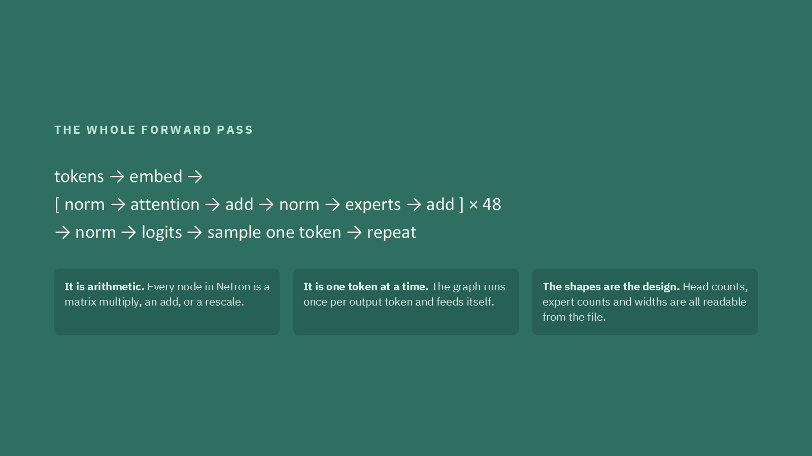
tokens → embed → [ norm → attention → add → norm → experts → add ] × 48 → norm → logits → sample one token → repeat

Three things follow from that line. It is arithmetic: every node in Netron is a matrix multiply, an add, or a rescale. It is one token at a time: the graph runs once per output token and feeds itself. And the shapes are the design: head counts, expert counts and widths are all readable from the file, which means claims about a model can be checked against the model.

Try it yourself

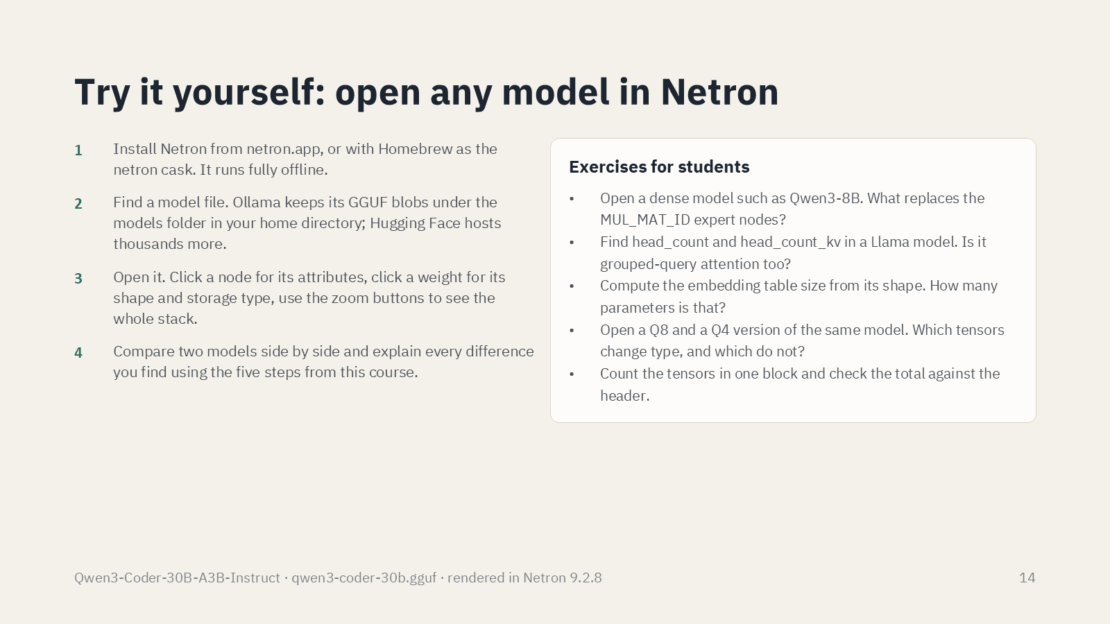
Netron installs from netron.app, or as the netron cask with Homebrew, and runs fully offline. Ollama keeps its GGUF blobs under the models folder in your home directory, and Hugging Face hosts thousands more. Open one, click a node for its attributes, click a weight for its shape and storage type, and use the zoom buttons to see the whole stack. For a large GGUF use the desktop app rather than the browser build, which loads the whole file into memory.

The exercises from the last slide escalate deliberately. The first two are reading, the third is arithmetic, the last two need two files side by side.

• Open a dense model such as Qwen3-8B. What replaces the MUL_MAT_ID expert nodes?
• Find head_count and head_count_kv in a Llama model. Is it grouped-query attention too?
• Compute the embedding table size from its shape. How many parameters is that?
• Open a Q8 and a Q4 version of the same model. Which tensors change type, and which do not?
• Count the tensors in one block and check the total against the header.

Every answer is verifiable by clicking. That is the point of teaching it this way.

Why this belongs on a security site

Australian businesses are being sold local models as the private alternative to a cloud API, and the pitch is usually made in words rather than tensors. Being able to open the file changes the conversation. The memory a model needs is its quantised size, not its parameter count. A context-window claim is a number in the header and a head count you can divide. "Open weights" means exactly this: the whole design is readable by anyone with a free viewer, which is true of the model you are evaluating and equally true of the one an attacker is running. A mental model of a transformer that is not just a citation of "attention is all you need" is the difference between assessing a vendor's claim and repeating it.